Final Project

|
|
The goal of this project was to better understand the transformation of 3D space into 2D images. I did this in two ways. I first transformed an object in 3D space onto a 2D image, this is the part that I reported on for the progress report due on April 26th. In the second part of the project, I added lines around objects selected by the user. These lines then propagated over the image until they were blocked by some other object at a different distance in the image. The latter part of this project was inspired by the work of Jim Sanborn, who was listed on the course website. I found Part 2 of the project more interesting, so most of the report focuses on these results.
Part 1 - Algorithm
The projection of an object onto a camera sensor depends on the properties of the camera, and the 3D position of the object relative to the camera. The algorithm must calculate the following: the position of the 3D object’s image on the sensor, the magnification of the object, and amount of blur of the object (this depends on the plane that the camera is focused and aperture of lens). The user specifies the following:
|
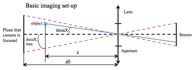
Xposition (or thetaX) – x position of object in 3D space relative to lens
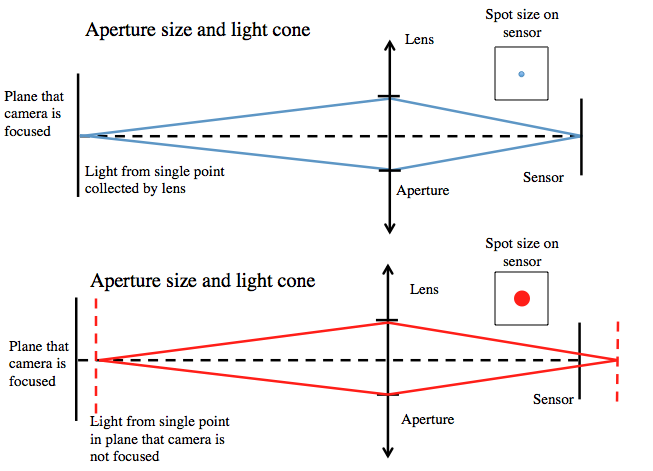
Xposition ( or thetaY) – y position of object in 3D space relative to lens z position – z position of object in 3D space relative to lens sensorX – size of sensor (horizontal) sensorY - size of sensor (vertical) aperture radius – radius of aperture stop in camera z0 – distance that camera is focused These figures show the geometry for determining where an object in space would be imaged onto a sensor. I am only showing the xz plane, but you can imagine extending this to the yz plane as well. As the aperture stop gets larger the amount of light collected by the camera increases. As a result the depth of field shrinks. Therefore, if the object is placed in a plane that the camera is not focused, then the spot size (blur of image) increases.
From this geometry, I wrote an algorithm for transforming an input image (the object) onto another image (the sensor). The image is blurred according to the size of the spot calculated, and then Poisson blending is used to blend the images together |
|
Part 1 - Results
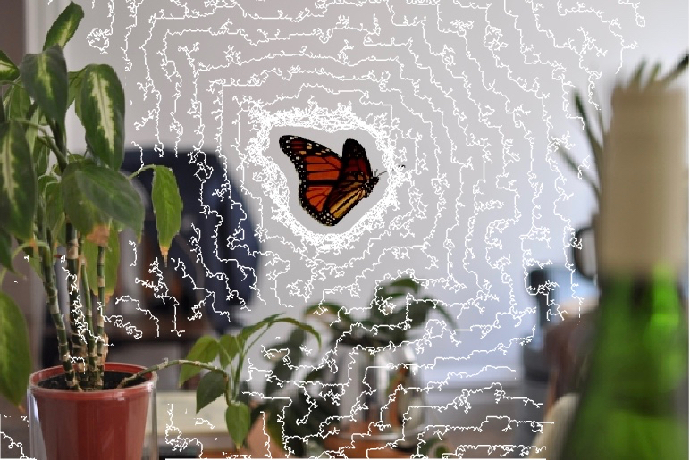
To test the algorithm, I set up a scene with plants positioned at different distances from the camera. A picture was then taken with a 50mm lens (f/#=1.8). The camera was focused at a position of 100mm (i.e. z0 = 100mm). I then selected an object (a picture of a butterfly) to be “imaged” by the camera using the algorithm. I chose several x,y,z positions to test. Here are some results. The max FOV given the sensor size and lens of camera was 6.7° by 4.5°
To test the algorithm, I set up a scene with plants positioned at different distances from the camera. A picture was then taken with a 50mm lens (f/#=1.8). The camera was focused at a position of 100mm (i.e. z0 = 100mm). I then selected an object (a picture of a butterfly) to be “imaged” by the camera using the algorithm. I chose several x,y,z positions to test. Here are some results. The max FOV given the sensor size and lens of camera was 6.7° by 4.5°
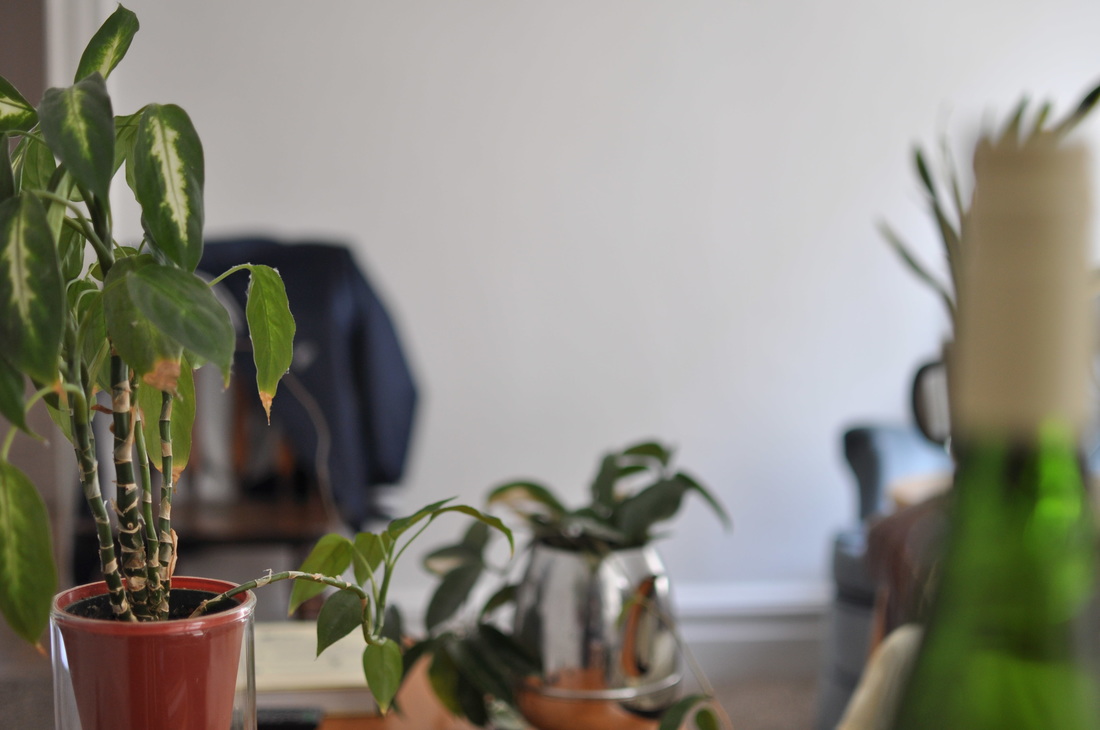
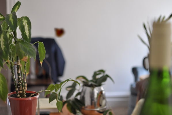
Original image of scene
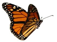
Original picture of object
|
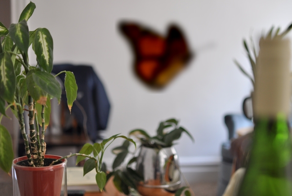
(thetaX, thetaY, z) = [2°, 2°, 230mm]
|
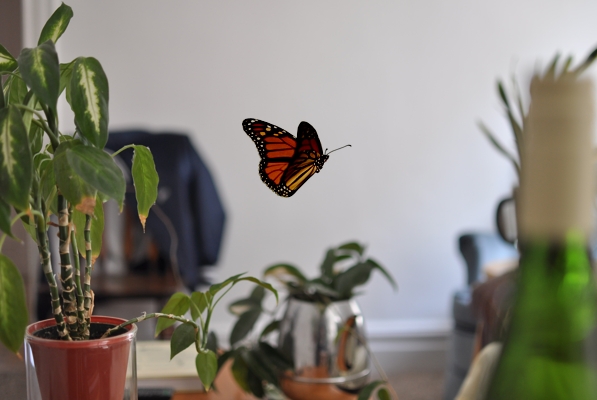
(thetaX, thetaY, z) = [0°, 1°, 100mm]
|
(thetaX, thetaY, z) = [-1°, 2°, 55mm]
|
|
I showed this initial result with the butterfly in the project update. Also shown here is a video of a green light moving through a trajectory that I created. This was inspired by the video synposis project I did in this class. To the right is a trajectory of the object in 3D space. The green point marks the start location and the red point marks the end location. You can click to move the plot to help visualize the trajectory. The video shows the 2D projection of that object onto a camera sensor as it travels through space and time. You can tell when the ball is the the plane that the camera is focused. Here are parameters that I set:
f=50; % focal length (mm) z0=200; % object distance - distance that camera is focused (mm) sy=6/2; % half vertical size of sensor (mm) sx=sy*4/3; % half horizontal size of sensor (mm) Arad=5; % aperture radius (mm) Part 1 - Analysis This part of the project reminds me of the paper presented in class called "Using Cloud Shadows to Infer Scene Structure and Camera Calibration," which cloud cover over time could be used to construct depth maps. I also aimed to understand the 2D representation of 3D world by adding an object to a scene at different depths. There were a ton of issues with this approach that led me to focus my time on Part 2 of the project. Firstly, it was really difficult to determine depth information computationally from a single image. In the paper mentioned above and during lecture, we learned a few cool ways to determine depth from static video. |
|
However, without some changing lighting element to the scene, I couldn't come up with an algorithm for determine depth of objects in the scene. This made it very difficult to test the algorithm without setting up a scene myself and knowing information about the camera. The results were also not that exciting. In the end, the output of the algorithm isn't much different than the results of the Poisson blending and gradient mixing assignment. The only difference is that some amount of blur and magnification is added to the object being pasted.
I originally thought about using this algorithm for synthesizing objects into video, like adding a moving object around some friend having a cup of coffee. The challenge in doing this was from the limitations of Poisson blending. If the object is to be pasted onto the existing image, then the background has to have low spatial detail. Note that I deliberately set up my scene with a white wall so that it would be easier to blend the butterfly onto the image. Due to these challenges, I shifted emphasis to Part 2 of project.
I originally thought about using this algorithm for synthesizing objects into video, like adding a moving object around some friend having a cup of coffee. The challenge in doing this was from the limitations of Poisson blending. If the object is to be pasted onto the existing image, then the background has to have low spatial detail. Note that I deliberately set up my scene with a white wall so that it would be easier to blend the butterfly onto the image. Due to these challenges, I shifted emphasis to Part 2 of project.
Part 2 - Algorithm
In this second part, I wanted to add interesting lines to images that accented objects at different depths in the image. This part most closely matches the work of Jim Sanborn's implied geometries series that was listed under the artistic side of computational photography descriptions on the site.
Segmentation
In order to add contour lines around objects at different depths, I needed to develop an algorithm for identifying and segmenting objects in the image. I wanted to automate the segmentation of objects instead of manually drawing lines around each object like we did in the Poisson blending project. There were two motivations for this: (1) I wanted the objects to be segmented very tightly around the boundary so that drawing lines around objects didn't look "blocky," and (2) I didn't want to take a lot of time for drawing outlines manually.
Again, I ran into problems with determining objects at different depths in a single image. Initially, I tried three techniques listed on Matlab: Otsu's method, K-means algorithm, and watershed segmentation. I chose the K-means algorithm for segmentation because it provided the most flexibility in determining how segmented the image was. Furthermore, Otsu and watershed methods specialized in segmenting objects with higher intensity relative to the background. Shown are the masks generated by each algorithm.
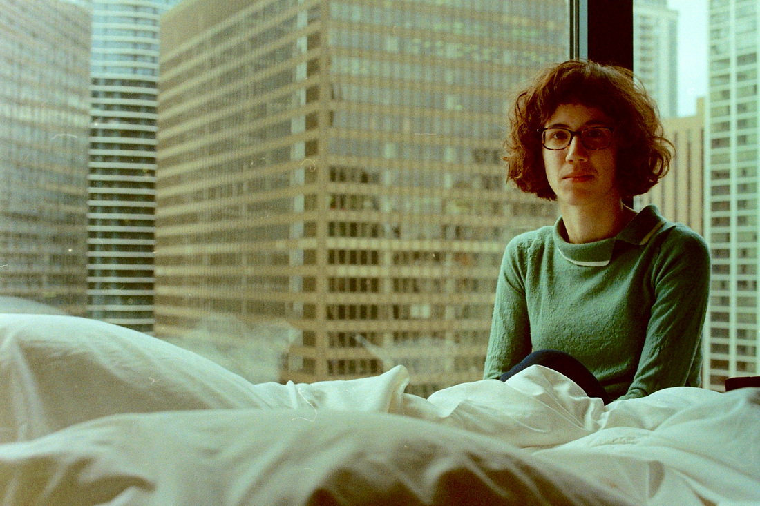
Original image

Segmentation using watershed method
|
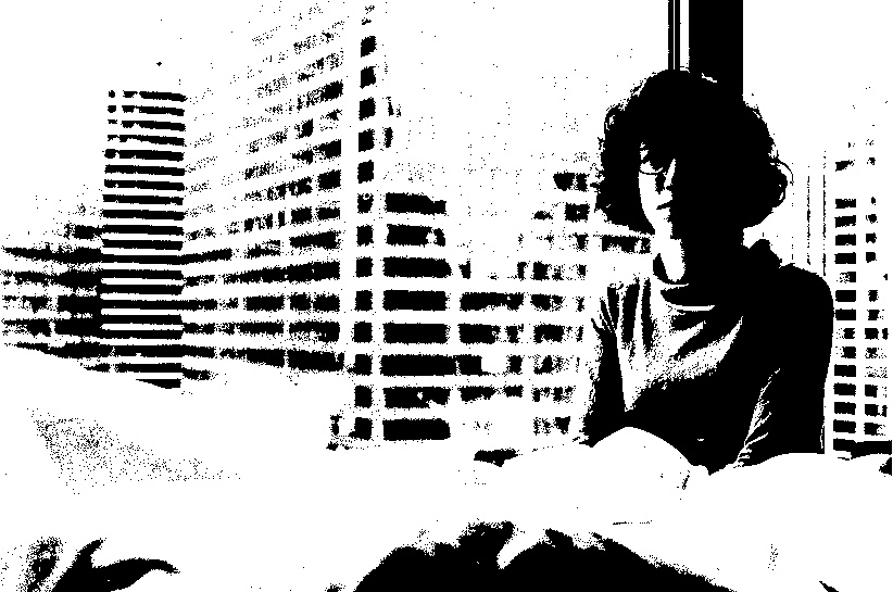
Segmentation using Otsu's method
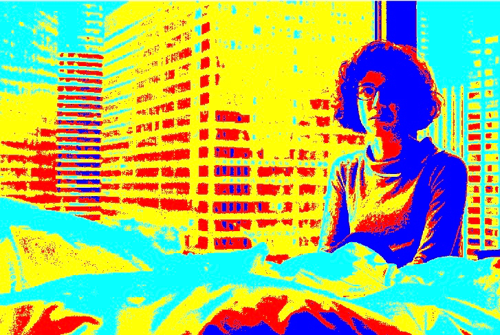
Segmentation using K-means method
|
Clearly the K-means segmentation would not be enough alone, so I added two additional components for segmentation: (1) additional user input to select the segments that made up the object of interest, and (2) the ability to fill segments that were on some boarder of the image. The algorithm also uses imclose to fill in the gaps of the mask so that the user doesn't have to get every segment that covers the object.
The user selects the number of clusters, the object to draw lines around, and any parts of the image that should be placed in the foreground or background. The more clusters selected, the more segments the image is broken up into and therefore the more likely it is that your object of interest is correctly separated from the rest of the image. However, the more clusters the more likely it is that your object is broken into many pieces.
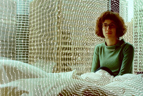
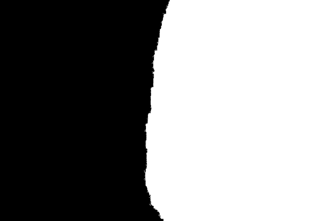
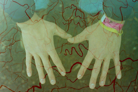
Shown below is the user interface for segmenting the images, as well as the masks for the object and the blanket that is in the foreground.
The user selects the number of clusters, the object to draw lines around, and any parts of the image that should be placed in the foreground or background. The more clusters selected, the more segments the image is broken up into and therefore the more likely it is that your object of interest is correctly separated from the rest of the image. However, the more clusters the more likely it is that your object is broken into many pieces.
Shown below is the user interface for segmenting the images, as well as the masks for the object and the blanket that is in the foreground.
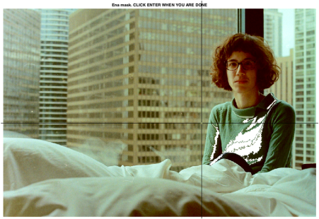
User interface: selecting segments for mask
|

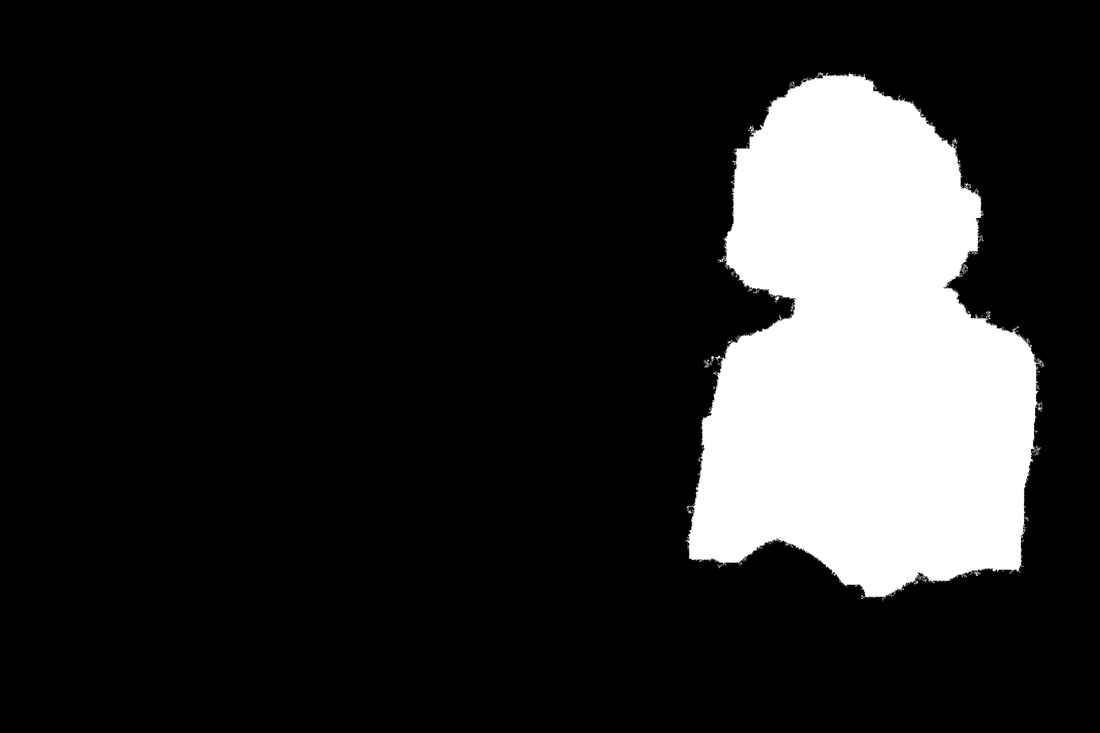
Mask before closing, which is creepy and cool
|
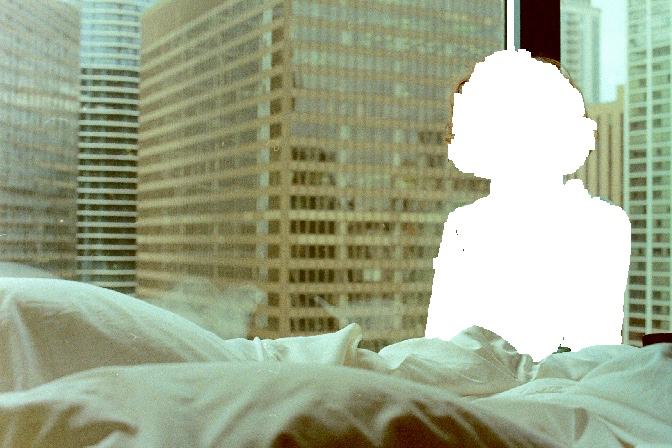
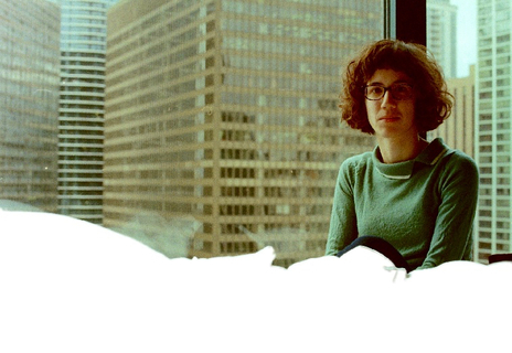
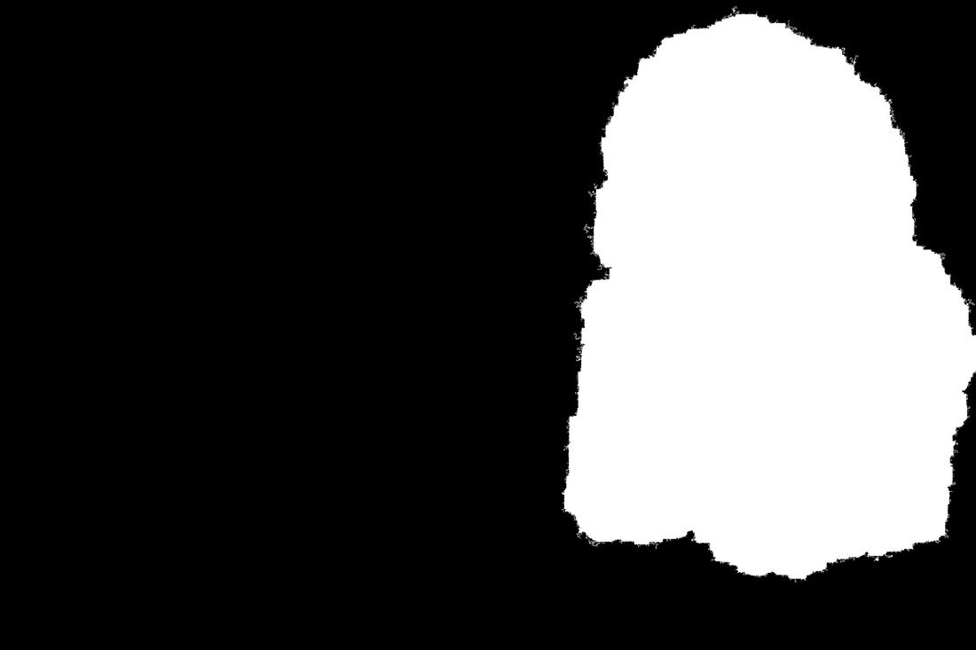
Final mask, after closing
|
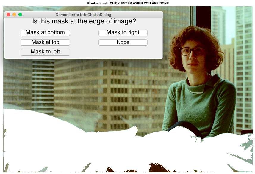
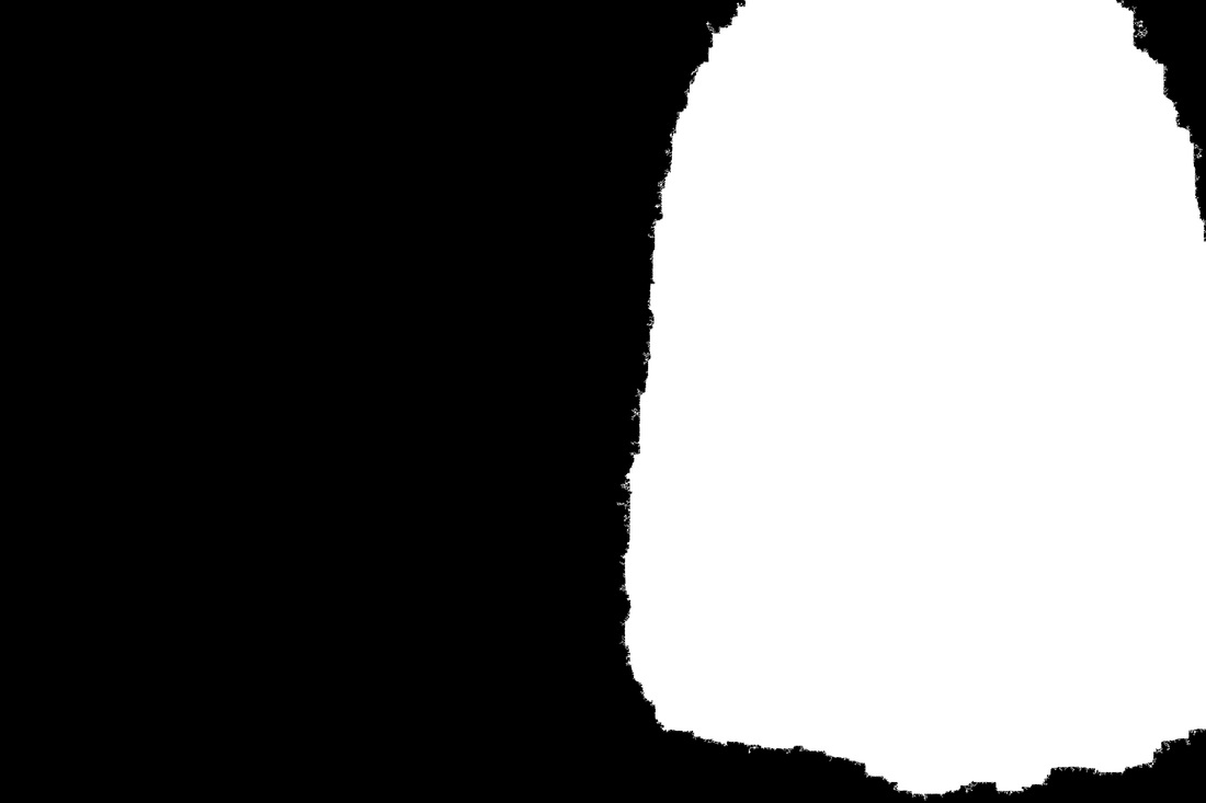
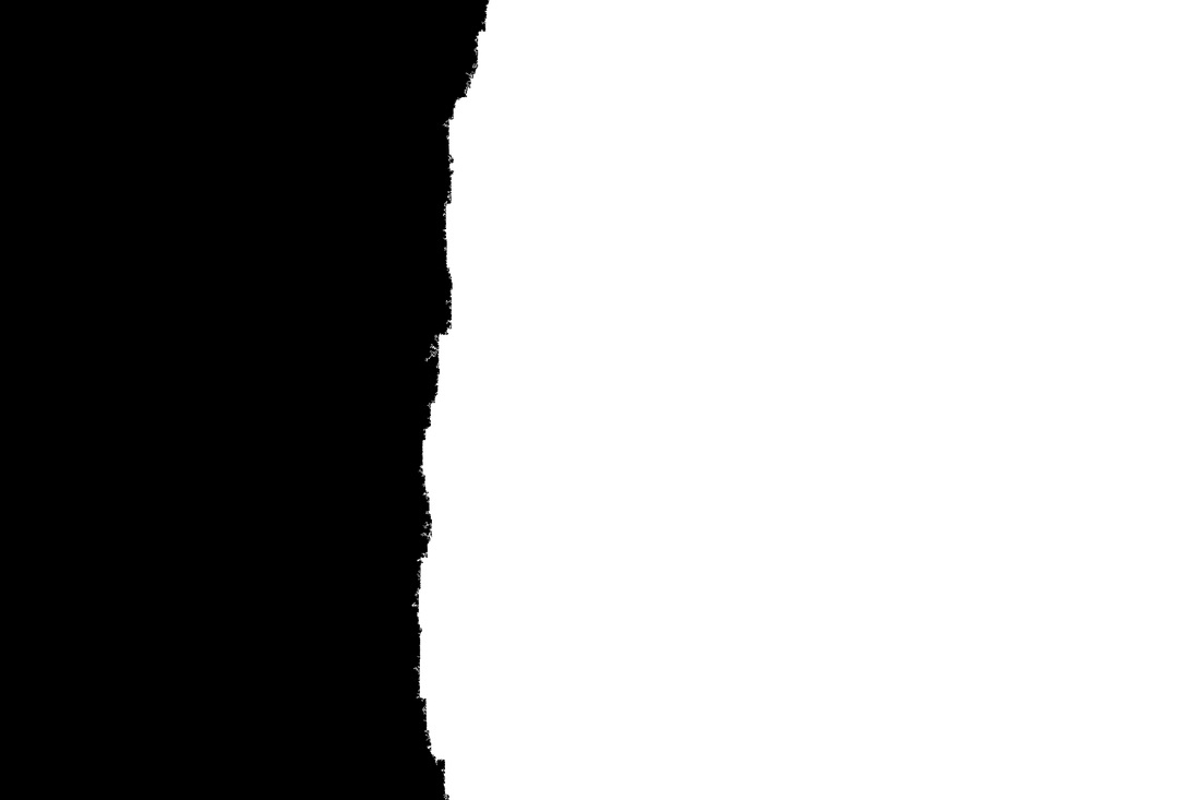
Program fills in holes if mask is at edge of image
|
Mask of blanket after using edge for completion
|
Drawing lines around objects
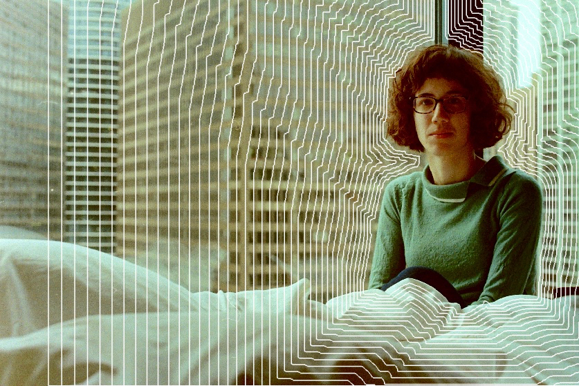
To draw lines around the object of the image, I found the boundary of the mask by using bwboundaries. Lines were added by increasing the size of the mask using either imdilate or an increasingly larger Gaussian filter. I didn't like how the lines looked initially because they appeared jagged, so I added noise to the mask before finding the boundaries. In this part of the algorithm, the user can select the spacing of the lines, the number of lines, the color of lines, the noisiness of the lines.
Finally, any parts of the image that were selected to be in the foreground were place back onto the image over top of the lines (e.g. the blanket).
Lines before adding noise
|
Lines after adding noise
|
|
|
Line masks
|
|
|
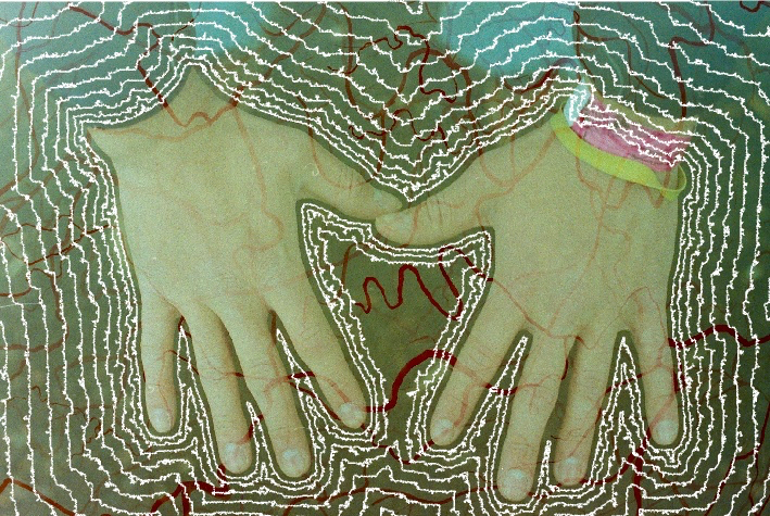
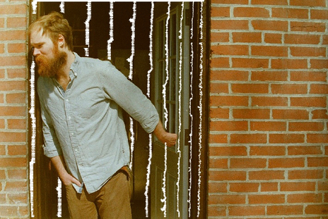
Part 2 - Results
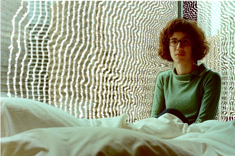
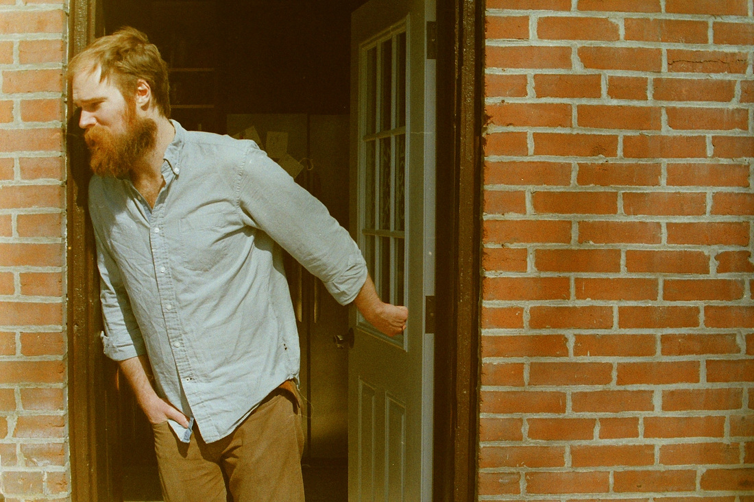
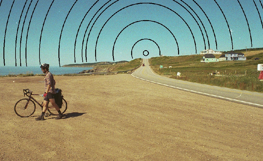
The algorithm was tested with several photos I took of my friends and family. I also included the photo I synthesized with the butterfly floating through the plants. The segmentation works pretty well across the images that I have shown. In the final example, I used vision.ShapeInserter to add circles to the sky instead of drawing lines around the object selected by the user.
The algorithm was tested with several photos I took of my friends and family. I also included the photo I synthesized with the butterfly floating through the plants. The segmentation works pretty well across the images that I have shown. In the final example, I used vision.ShapeInserter to add circles to the sky instead of drawing lines around the object selected by the user.


|

|
Part 2 - Analysis
The algorithm is working as I imagined, although there isn't too much function besides creating cool looking images. I think you can definitely see the inspiration of Jim Sanborn's work in the results. The key difference is that his lines look like they are projections onto the objects. You can see the lines matching the grooves and rocks of the canyons. I also used images with people, whereas he focused on images of landscapes.
Biggest weakness in the algorithm is the segmentation. The amount of user input isn't ideal, and sometimes there are errors that you can probably notice in the results. I think it would be nice to add addition features for line drawing, similar to the circles added in the last example. I also was thinking of creating videos of the line propagating over the images. Some of this code could also be useful for that advertisement company that visited the class. By segmenting different parts of the image at different distances and using parts of the 3D to 2D transform code, you may be able to create those moving gif-like images that they showed us.